Although Diffusion Model is a new generative framework, it still has many shades of other methods.

Generation & Diffusion

Just like GANs realized the implicit generation through the mapping from a random gaussian vector to a natural image, Diffusion Model is doing the same thing, by multiple mappings, though. This generation can be defined as the following Markov chain with learnable Gaussian transitions:

$$ \begin{align} p_\theta\left(x_0\right)=\int p_\theta\left(x_{0: T}\right) \mathrm{d} x_{1: T}\\ p_\theta\left(x_{0: T}\right):=p_\theta\left(x_T\right) \prod_{t=1}^T p_\theta\left(x_{t-1} \vert x_t\right)\\ p_\theta\left(x_{t-1} \vert x_t\right):=N(x_{t-1};\mu_{\theta}(x_t,t),\Sigma_\theta(x_t,t)) \end{align} $$

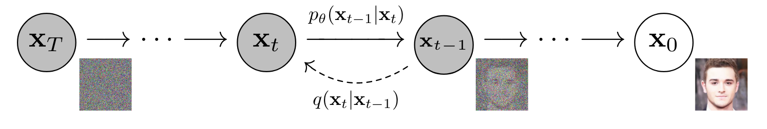
Markov chain: What happens next depends only on the state of affairs now. So we have $p(x_{t-1}\vert x_{t:T})=p(x_{t-1}\vert x_{t})$

Similar to VAE, we can use the posterior $q(x_{1:t} \vert x_0)$ to do the estimation for $\theta$. The difference is that $x_1,\dots,x_T$ are the latents of the same size as $x_0$, and the diffusion process (c.t. VAE encoder) $q(x_{1:T} \vert x_0)$ is fixed to a Markov chain without any learnable parameters, which can be designed as Gaussian transitions parameterized by a decreasing sequence $\alpha_{1:T}\in [0,1]^T$:

$$ \begin{align} q(x_{1:T} \vert x_0) := \prod_{t=1}^T q\left(x_{t} \vert x_{t-1}\right) \\ q(x_t \vert x_{t-1}):=N(\frac{\sqrt{\alpha_t}}{\sqrt{\alpha_{t-1}}}x_{t-1}, (1-\frac{\alpha_t}{\alpha_{t-1}})I) \end{align} $$

A nice property of the above design (thank to Gauss.) is that it admits sampling $x_t$ at arbitrary timestep $t$:

$$ q(x_t\vert x_0)=N(x_t;\sqrt{\alpha_t}x_0, (1-\alpha_t)I) $$

Training Objective

We can use the variational lower bound (appeared in VAE) to maximize the negative log-likelihood:

$$ \max_{\theta}E_{q}[\log{p_\theta(x_0)}]\leq \max_{\theta}E_{q}[\log{p_{\theta} (x_{0:T})}-\log{q(x_{1:T} \vert x_0)}] $$

which also can be driven by Jensen’s inequality as in Lil’log. And we can further rewrite this object as:

Using Bayes’ rule, we can deduce the fact that $q(x_{t-1}\vert x_t, x_0)$ is also a gaussian distribution.

where $L_T$ is constant. Discussing $L_{t-1}$ is one of the key contributions of DDPMs. If generative variances is all fixed $\Sigma_t = \sigma^2_t$, using parameterization (fit distribution $\to$ fit mean $\to$ predict noise) and reweighting based on the empirical results, we can simplify this objective as follows:

$$ L_t=E_{x_0\sim q, \epsilon\sim N(0,1)}\left[|| \epsilon_\theta(\sqrt{\alpha_t}x_0+\sqrt{1-\alpha_t}\epsilon, t)-\epsilon {||}_2^2 \right] $$

NCSN vs DDPM, different ways lead to almost the same objective!

For last $L_0$, DDPMs treat it as an independent discrete decoder derived from $N(x_0;\mu_{\theta}(x_1,1), 0)$, so it can be trained by the same objective as $L_t$. Notice that this last generative process is set to noiseless to ensure the lossless codelength of discrete data.

At the end, we can realize the efficient training by optimizing random terms of $L_t$ with stochastic gradient descent (Alg. 1). Correspondingly, the sampling can be exported by $p_\theta(x_{t-1}\vert x_t)$ using predicted $\epsilon_\theta(\cdot)$ (Alg. 2).

DDPM+

Finding 1: Why fixing $\sigma^2$ to $\beta$ or$\tilde{\beta}$ achieve similar sample quality?

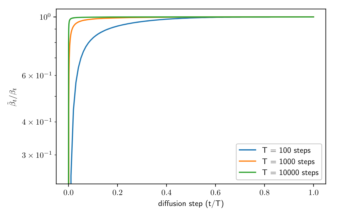
As $\beta \approx \tilde{\beta}$ In the early process, the perceptual details generated from these two is very similar. So the other constants might not matter at all for sample quality due to decreasing nature $\frac{\beta_t}{\beta_{t-1}} \to 0$.

Finding 2: The diffusion samples from linear schedule lose information very quickly.

In the diffusion process, these samples will soon become the noise without any information. Even if the early generation is skipped (~20%), the quality does not get much worse. It suggests that so much full noisy samples might do not contribute to generation.

Improvements

• Learnable variances with an interpolation between $\beta$ and $\tilde{\beta}$, driven by loss $+ \lambda L_{vlb}$.
• Cosine schedule has a linear drop off in the middle of the process, while changing very little near the start and the end.
• Resampling $L_{vlb}$ to make training stable (like a kind of dynamic weighting)

DDIM

More free diffusion chain

In DDIM, the authors introduce a extended version $q(x_{t-1}\vert x_t, x_0)$, which has the same marginal noise distribution $q(x_{t}\vert x_0)$：

$$ q_{\sigma}(x_{t-1} \vert x_t, x_0) = N(x_{t-1}; \sqrt{\alpha_{t-1}} x_0 + \sqrt{1 - \alpha_{t-1} - \sigma_t^2} \frac{x_t - \sqrt{\alpha_t} x_0}{\sqrt{1 - \alpha_t}}, \sigma_t^2 I) $$

Therefore, the corresponding generative process can be exported as:

Acceleration via subsampling

In the generation, we sample a subset of S steps ${\tau_1,\dots,\tau_S}$ to form a new chain as:

$$ q_{\sigma, \tau}(x_{\tau_{i-1}} \vert x_{\tau_i}, x_0) = N(x_{\tau_{i-1}}; \sqrt{\alpha_{\tau_{i-1}}} x_0 + \sqrt{1 - \alpha_{\tau_{i-1}} - \sigma_t^2} \frac{x_{\tau_i} - \sqrt{\alpha_{\tau_i}} x_0}{\sqrt{1 - \alpha_{\tau_i}}}, \sigma_{\tau_i}^2 I) $$

which can still provide high-quality samples using a much fewer number of steps.

References

• Jonathan Ho, Ajay Jain, and Pieter Abbeel, ‘Denoising Diffusion Probabilistic Models’, in Advances in Neural Information Processing Systems, 2020.
• Alexander Quinn Nichol and Prafulla Dhariwal, ‘Improved Denoising Diffusion Probabilistic Models’, in Proceedings of the 38th International Conference on Machine Learning, 2021.
• Jiaming Song, Chenlin Meng, and Stefano Ermon, ‘Denoising Diffusion Implicit Models’, in International Conference on Learning Representations, 2021.