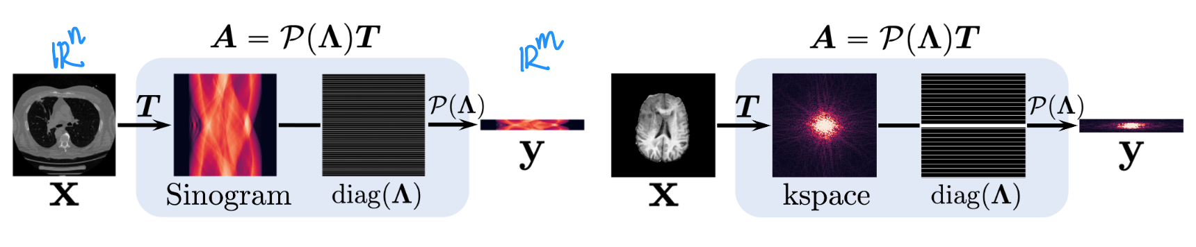
“An inverse problem seeks to recover an unknown signal from a set of observed measurements. Specifically, suppose $x\in R^n$ is an unknown signal, and $y\in R^m = Ax+z$ is a noisy observation given by m linear measurements, where the measurement acquisition process is represented by a linear operator $A\in R^{m\times n}$, and $z\in R^n$ represents a noise vector. Solving a linear inverse problem amounts to recovering the signal $x$ from its measurement $y$. Without further assumptions, the problem is ill-defined when $m< n$, so we additionally assume that $x$ is sampled from a prior distribution $p(x)$”

source from Dr. Yang Song’s paper

As unconditional generative model, Diffusion models (or Score models) can play a prior term in optimization for various ill-posed image inverse problems. Such methods are often labeled as training-free, zero-shot, unsupervised, etc.

On the other hand, Diffusion models also can be trained as conditional one $s_\theta(x_t,y,t)$, where $y$ is the condition from other mode. However, this will consume a lot of resources both in the computing power and the collection of paired data $\lbrace x_i,y_i\rbrace$.

Medical Score-SDE

-> Yang Song, et al. in ICLR, 2022.

step1: Perturbing measurements

Since $x_t=\alpha(t)x_0+\beta(t)z$, and we set $y_t=Ax_t+\alpha(t)\epsilon$, so we have $y_t=\alpha(t)y+\beta(t)Az$.

Smart and reasonable assumption for the coefficient $+\alpha(t)\epsilon$ to avoid the subsequent diffusion of random measurement noise $\epsilon$.

step2: Generation with Score-SDE

Using the Euler-Maruyama sampler, the generative process given by:

$$ x_{t-\Delta t} = x_t-f(t)x_t\Delta t+g(t)^2s_\theta(x_t,t)\Delta t+g(t)\sqrt{\Delta t}z $$

where $s_\theta(\cdot)$ is the trained score model, $\Delta t = 1/N$ is the set discrete time, and $z\sim \mathcal{N}(0,1)$.

step3: Consistent Guidance

$$ \begin{aligned} x_t^{\prime}&=\arg \min_{v\in R^n}\lbrace (1-\lambda)\Vert v-x_t \Vert_{T}^2 + \min_{u\in R^n} \lambda \Vert v-u \Vert_{T}^2 \rbrace \ s.t.\quad Au&=y_t \end{aligned} $$

which has the closed-form solution as:

$$ x_t^{\prime}=T^{-1}[\lambda \Lambda \mathcal{P} ^{-1}(\Lambda)y_t+(1-\lambda)\Lambda Tx_t+(1-\Lambda)Tx_t] $$

When the measurement process is noisy, we can choose $0<\lambda<1$ to allow slackness in $Ax_t^{\prime}=y_t$ (more affected by $p(x)$). When the measurement process contains no noise, the authors chosse $\lambda=1$ at the last sampling step to guarantee $Ax_0^{\prime}=y$.

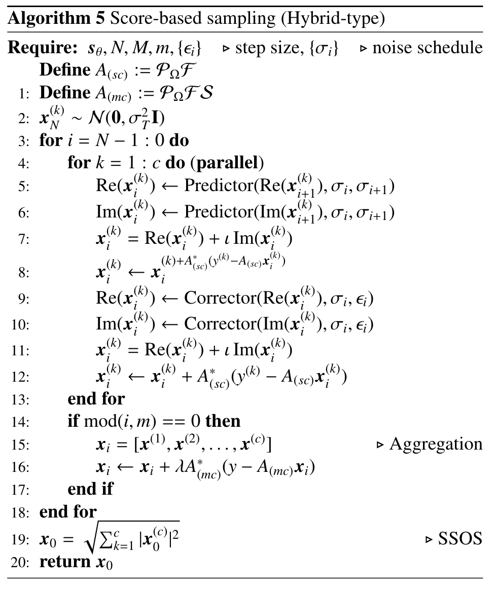
Score-MRI

-> Hyungjin Chung, et al. Medical Image Analysis, 2022.

Similar to the above, Score-MRI inserts a more simple consistency mapping after every “Predictor” and “Corrector” iteration.

$$ x_i=x_i+\lambda A^\ast(y-Ax_i)=(I-\lambda A^\ast A)x_i+A^\ast y $$

where $A^\ast$ denotes the Hermitian adjoint, and $+\lambda A^\ast (y-Ax_i)$ can be viewed as a rectification for minimizing the distance between $y$ and $Ax_i$. In the hybridtype Algorithm 5 (complex domain and multi-coils for MRI), the authors start with $\lambda = 1.0$ in the first iteration, and linearly decrease the value to $\lambda=0.2$ at the last iteration.

GANCS has an similar rectification $(I-\Phi^{†}\Phi)x+\Phi^{†}y$, where pseudo-inverse $\Phi^{†}$ satisfies $\Phi\Phi^{†}\Phi=\Phi$, but without the scaling factor $\lambda$. In this paper, the authors view $(I-\Phi^{†}\Phi)x$ as a projection onto the nullspace of $\Phi$.

DDNM

-> Yinhuai Wang, et al. in ICLR, 2023.

Noise-free

Similar to GANCS, DDNM adopts a rectified estimation as:

$$ x_{0|t}^{\prime}=A^{†}y+(I-A^{†}A)x_{0|t} $$

where $x_{0|t}$ is the predicted version at timestep $t$. Based on DDIM, the generative process can be driven by $x_{t-1}\sim \mathcal{p}(x_{t-1}|x_t,x_{0|t}^{\prime})$. So it might provide a more reliable rectification to human-perceptible $x_{0|t}$, rather than noisy $x_t$ like in Score-MRI.

Although this paper mentioned that this consistency mapping was inspired by range-null space decomposition $x=A^{†}Ax+(I-A^{†}A)x$, but it seems to contradict with the subsequent DDNM+ for the noisy inverse problem.

Noisy

$$ x_{0|t}^{\prime}=A^†y+(I−A^†A)x_{0|t} =x_{0|t}-A^†(Ax_{0|t}-y) $$

In short, the authors employ two scale factors $\Sigma_t$ & $\Phi_t$ into range-space correction & generative variance, respectively.

$$ \begin{aligned} x_{0|t}^{\prime}&= x_{0|t}-\Sigma_tA^†(Ax_{0|t}-y)\\ p^{\prime}(x_{t-1}|x_t,x_{0|t}^{\prime})&=\mathcal{N}(x_{t-1};\mu_t(x_t, x_{0|t}^{\prime}),\Phi_t I) \end{aligned} $$

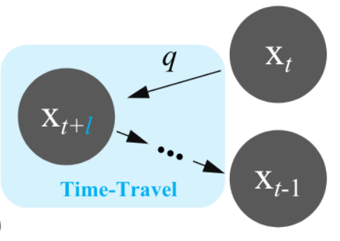
However, the performance gains from these factor are not clear, due to the absence of ablations experiments. It looks like the “Time-Travel” (a kind of redundant computing) helped a lot.

References

• Yang Song and others, ‘Solving Inverse Problems in Medical Imaging with Score-Based Generative Models’ in International Conference on Learning Representations, 2022.
• Hyungjin Chung and Jong Chul Ye, ‘Score-Based Diffusion Models for Accelerated MRI’, Medical Image Analysis, 80 (2022), 102479.
• Johannes Schwab, Stephan Antholzer, and Markus Haltmeier, ‘Deep Null Space Learning for Inverse Problems: Convergence Analysis and Rates’, Inverse Problems, 35.2 (2019), 025008.
• Morteza Mardani and others, ‘Deep Generative Adversarial Networks for Compressed Sensing Automates MRI’ arXiv, 2017.
• Yinhuai Wang, Jiwen Yu, and Jian Zhang, ‘Zero-Shot Image Restoration Using Denoising Diffusion Null-Space Model’ in International Conference on Learning Representations, 2023.