Both likelihood-based methods and GAN methods have have some intrinsic limitations. Learning and estimating Stein score (the gradient of the log-density function $\nabla_{ x} \log p_{\text {data }}( x)$) may be a better choice than learning the data density directly.

Score Estimation (for training)

We want to train a network $s_{\theta}(x)$ to estimate $\nabla_{ x} \log p_{\text {data }}( x)$, but how can we get the ground truth (the real score)? In this paper, the objective $\frac{1}{2} E_{p_{\text{data}}} \lbrack\lVert s_{\theta}( x)-\nabla_{ x} \log p_{\text{data}}( x)\rVert_2^2\rbrack$ is equivalent to the following by Score Matching:

$$ E_{p_{\text{data}}}\left[tr(\nabla_{ x}s_{\theta}( x))+\frac{1}{2}\left|s_{\theta}( x))\right|_2^2\right] $$

Unfortunately, it is not easy to compute $tr(\cdot)$ for a large-scale problem. Both Denoising score matching and Sliced score matching are popular methods to deal with this situation. But the sliced one requires 4x computations due to the forward mode auto-differentiation. Instead, Denoising score matching try to estimate the score of noise-perturbed distribution ($q_\sigma$) as follows:

$$ \frac{1}{2} E_{q_\sigma(\tilde{ x} \mid x) p_{\text {data }}( x)}\left[\left| s_{\theta}(\tilde{ x})-\nabla_{\tilde{ x}} \log q_\sigma(\tilde{ x} \mid x)\right|_2^2\right] $$

Minimizing this objective, we can get $s_{\theta}( x)=\nabla_{ x} \log q_{\sigma}( x)$. And if the noise is small enough $q_\sigma( x) \approx p_{\text {data }}( x)$, we will get $s_{\theta}( x)=\nabla_{ x} \log q_\sigma( x) \approx \nabla_{ x} \log p_{\text {data }}( x)$. As $q_\sigma(\tilde{x}| x)$ can be defined as a known simple distribution, this minimization is easier than regular score matching. In this paper, they choose $q_\sigma(\tilde{x}| x) =N\left(\tilde{x} \mid x, \sigma^2 I\right)$, which leads to:

$$ \ell(\theta ; \sigma) \triangleq \frac{1}{2} E_{p_{\text {data }}(x)} E_{\tilde{x} \sim N\left(x, \sigma^2 I\right)}\left[\left|\mathbf{s}_{\theta}(\tilde{x}, \sigma)+\frac{\tilde{x}-x}{\sigma^2}\right|_2^2\right] $$

Langevin dynamics (for inference)

How can we do sampling from $p_{\text {data }}( x)$ when we get a nice estimation of $\nabla_{ x} \log p_{\text {data }}( x)$? Just along the direction of this gradient? Yes, but plus more tricks.

$$ x_t = x_{t-1}+\frac{\epsilon}{2} \nabla_{x} \log p\left(x_{t-1}\right)+\sqrt{\epsilon} z_t $$

The Annealed Langevin dynamics, which is based on assumptions for particle motion, can provide more stable distribution! Briefly, the random noise term $\mathbf{z}_t \thicksim N(0,1)$ simulates the random motion of particles. With gradual annealing (the step size $\epsilon \to 0$), the iterative $x_t$ will approach the distribution $p(x)$.

Practical Challenges

The manifold hypothesis

The data in the real world tend to concentrate on low dimensional manifolds embedded in a high dimensional space (a.k.a., the ambient space).

• The score is undefined.
• The estimation by Score Matching isn’t consistent.

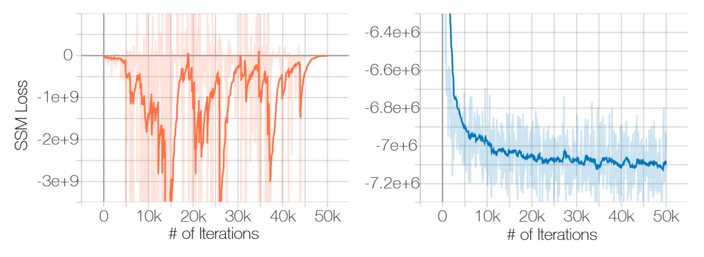
If we perturb the data with a small Gaussian noise (make the support of data distribution is the whole space), the loss driven by SlicedScoreMatching (fast & faithful) will converge (Fig. 1).

Low data density regions

Our training is based on the data in high density ($\thicksim p_{\text {data }}( x)$).

• The estimation in low density regions is inaccurate.
• Regular Langevin Dynamics can’t be able to correctly recover the relative weights of the multi-modal distribution in reasonable time.

If we perturb the data by using multiple noise levels (anneal down), we can fill the low density regions.

So naturally, we can kill three birds with Denoising Score Matching! Large-scale estimation, Whole space support, and Filling low density regions. (Indeed, the authors emphasize that empirically sliced score matching can train NCSNs as well as denoising score matching.)

One More Thing

In the score matching, the authors approximately have $\left| s_{\theta}( x, \sigma)\right|_2 \propto 1 / \sigma$, so they choose $\lambda (\sigma) = \sigma^2$ to make the order magnitude of loss under various noise levels roughly the same, and independent of $\sigma$.

$$ \mathcal{L}\left(\theta ;\lbrace\sigma_i \rbrace_{i=1}^{L}\right) \triangleq \frac{1}{L} \sum_{i=1}^L \lambda\left(\sigma_i\right) \ell\left(\theta ; \sigma_i\right) $$

Correspondingly, in the langevin dynamics, they choose $\alpha_i \propto \sigma^2$ to make the order magnitude of “signal-to-noise ratio” independent of $\sigma$.

References

• Yang Song and Stefano Ermon, ‘Generative Modeling by Estimating Gradients of the Data Distribution’, in Advances in Neural Information Processing Systems, 2019.
• Yang Song and others, ‘Score-Based Generative Modeling through Stochastic Differential Equations’, in International Conference on Learning Representations, 2021.