Controllable Text-To-Image (T2I) generation has always been a major challenge in diffusion models. On the one hand, people hope that the generated images can follow some predefined physical attributes, such as the number, position, size, and texture of objects. On the other hand, they also require the T2I models to retain a certain level of creativity.

At present, there are quite a lot of researches related to controllable T2I generation. I prefer to divide them into two categories: one primarily focuses on correcting the generation path in inference, called Explicit Control; the other one strengthens the network through fine-tuning or adding new layers, called Implicit Control.

This blog, as the first part of this series, will summarize representative researches related to Explicit Control, which can be further divided into two technical routes: forward guidance and backward guidance. The discussion of implicit control will be updated in another blog post.

PS: This explicit or implicit statement comes from my personal preference and is not yet widely accepted in the academic community.

Early Explorations before the Stable Diffusion

Image-to-Image & Inpainting

-> Chenlin Meng, et al. arXiv 2021

-> Andreas Lugmayr, et al. CVPR 2022

The idea of explicit control can date back to before the Stable Diffusion, with two classic examples being SDEdit (Image-to-Image) and RePaint (Inpainting). Due to their relatively simple principles, here we just briefly summarize them:

SDEdit uses a noisy version of a reference image as the starting point for the denoising process, ensuring that the generated image maintains a similar color layout to the reference image. Repaint, during the denoising process, combines the masked background image with the predicted foreground image to realize inpainting new content in the masked regions.

Both of these classic methods achieve controllable generation through modify denoising process (without any training), demonstrating the strong robustness of the diffusion model and the significant potential for modifying the denoising process manually!

In the Diffusers library, the StableDiffusionInpaintPipeline has two versions. The unfinetuned version is based on the idea of Repaint without training, while the finetuned version involves concatenating the Mask and Masked_image_latents as additional 5 channels to the input of Unet and fine-tuning all layers. The latter version achieves better results.

Blended Diffusion

-> Omri Avrahami, et al. CVPR 2022

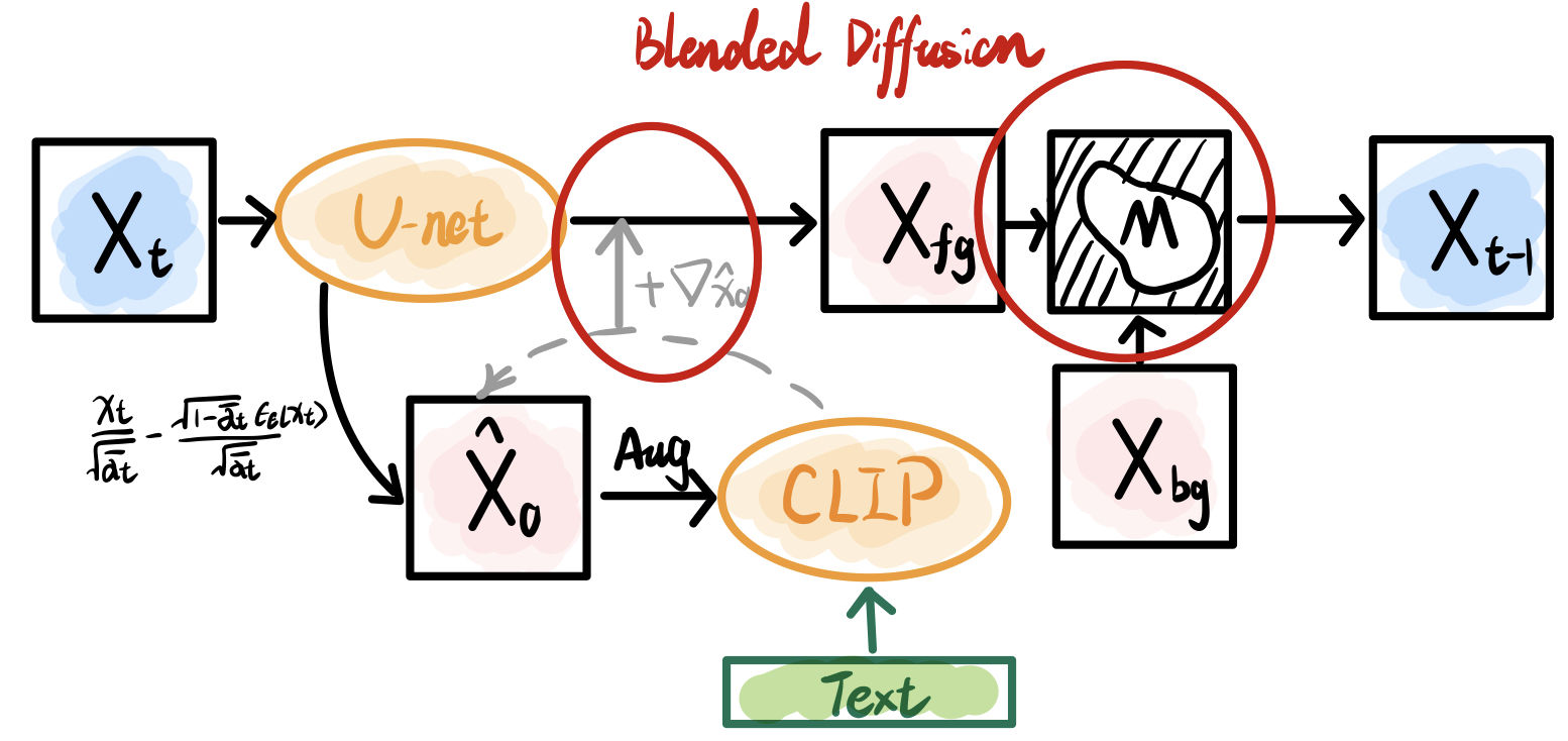
With the introduction of CLIP technology, Blended Diffusion achieves text-driven inpainting. The basic approach can be summarized as above figure. In each iteration, $\hat{x_0}$ is predicted based on the inverse equation of the known $p(x_t|x_0)$, and is masked accordingly. Then, the masked image and the text prompt are jointly input into CLIP to obtain a cosine similarity score $\mathcal{L}$ (with the trick of data augmentation to improve sensitivity). The gradient of this score is used to update the latent $\epsilon(x_t)+\nabla_{\hat{x_0}}\mathcal{L}$. Moreover, the foreground and background images are fused based on the given mask to update the latent $x_{t-1}$ for next iteration.

This approach is essentially a combination of CLIP-based T2I and Repaint method. In fact, the CLIP-based generation is a kind of classifier-based guidance, where the iteration values are updated based on the gradient of a certain criterion. Although this gradient-based approach may sound a little old-school in the days of Classifier-Free Guidance (CFG), we can still see its effectiveness in serval cutting-edge studies later on.

Forward Guidance

Prompt-to-Prompt Image Editing with Cross Attention

-> Amir Hertz, et al. arXiv 2022

Prompt-to-Prompt (P2P) focuses on editing already generated images, which may not be relevant to controllable generation, but it shows great potential of manipulating Cross Attention (CA) maps and brings quite a lot of inspiration to controllable generation techniques!

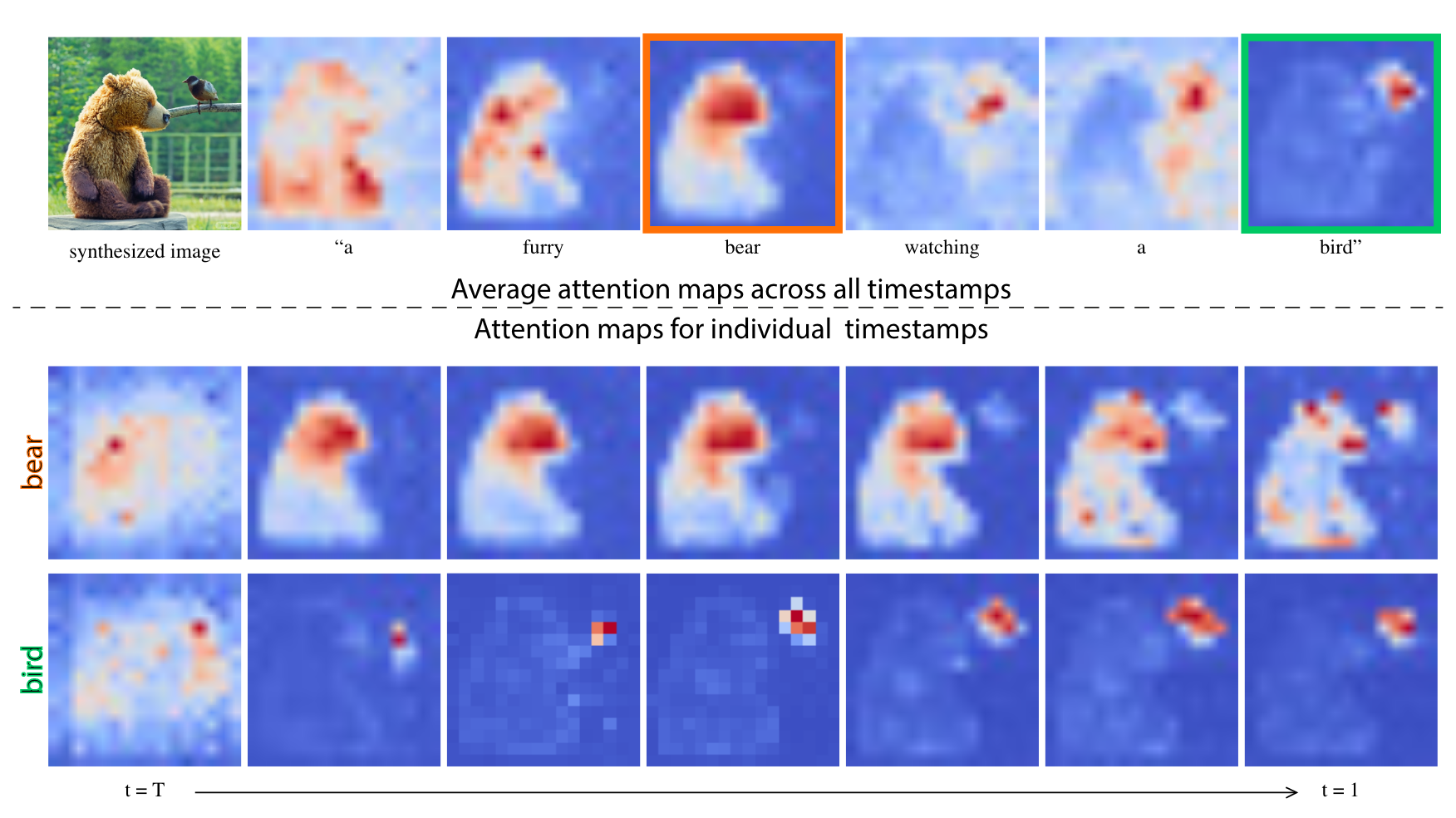
As shown above, P2P first found that CA corresponding to text tokens had strong semantic information (even in the early stages of generation). This finding seems obvious when you realize that CA is the similarity between image features and text features. But no one had visualized them before, and such strong semantic connections were not well known!

At the same time, this observation also reveals how the CA mechanism drives T2I generation. Let’s imagine the data flow: the sequence of text features from CLIP is first mapped to base values, then fused at different locations based on attention weights (the similarity between images and texts), and finally makes up the image we see (magical multimodal learning)!

More excitingly, the authors successfully controlled generation by manipulating CA values:

• Replacing the CA corresponding to a text token for content replacement.
• Deleting the CA corresponding to a text token for content erasure.
• Adding the CA corresponding to a text token for content addition.
• Weighting the CA corresponding to a text token to effectively enhance or weaken content.

Now we can enhance or weaken the content by weighting the text features from CLIP directly. This “weighted prompt” trick is widely integrated into various T2I tools (such as compel, A1111-webui, Midjourney, etc.).

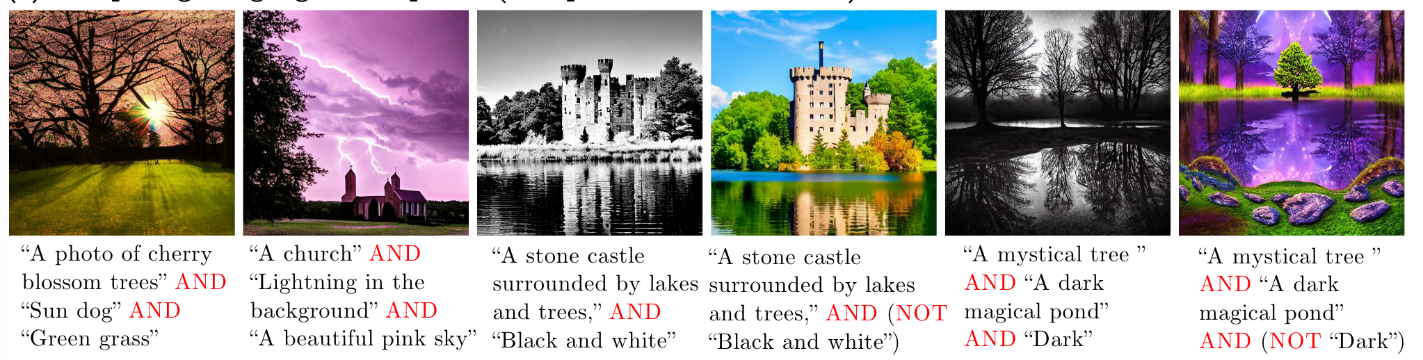
Compositional Visual Generation with Composable Diffusion Models

-> Nan Liu, et al. ECCV 2022

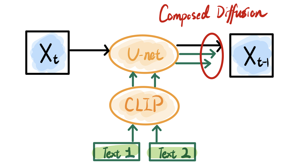
Composed Diffusion supports the generation of more content or objects. Although this paper is inspired by composing multiple EBMs, this idea is equivalent to the advanced CFG formally. In short, multiple text prompts separated by the “AND” symbol are fed into the diffusion model separately and then weighted to produce the results:

$$ \hat{\epsilon}(x_t,t)=\epsilon(x_t,t)+\sum_{i=1}^{n}w_i(\epsilon(x_t,t|c_i)-\epsilon(x_t,t)) $$

This synthesis is a bit crude and often less than expected, because different content will merge globally without explicit location constraints. Therefore, Composed Diffusion is more suitable for those multi-content with large spatial differences to avoid unexpected conflicts.

MultiDiffusion: Fusing Diffusion Paths for Controlled Image Generation

-> Omer Bar-Tal, et al. arXiv 2023

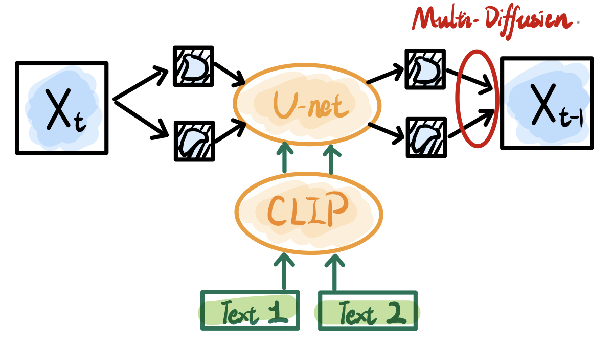
If we want more control over spatial position, the most direct way is to draw something in a certain region by specifying a target mask or box. While this sounds like a multi-region inpainting task, the question is how to ensure that they are independent and harmonious with each other?

MultiDiffusion gives the answer. The authors first build a mathematical optimization model for harmonious multi-region generation and derive a closed-form solution:

$$ \begin{align} \Psi\left(J_t \mid z\right)=\arg\min_{J\in\mathcal{J}}\sum_{i=1}^n\left|W_i \otimes\left[F_i(J)-\Phi\left(I_t^i \mid y_i\right)\right]\right|^2 \\ \Psi\left(J_t \mid z\right)=\sum_{i=1}^n \frac{F_i^{-1}\left(W_i\right)}{\sum_{j=1}^n F_j^{-1}\left(W_j\right)} \otimes F_i^{-1}\left(\Phi\left(I_t^i \mid y_i\right)\right) \end{align} $$

In fact, MultiDiffusion can be understood as a multi-region extension of Repaint. It fuses multiple images generated from different regions (depending on the degree of overlap) in each step, and then eliminates dissonance at the boundaries solely by the robustness of the denoising process. Obviously, due to the lack of interaction between the central features of different regions, the final generated image has obvious style variations across regions.

The derived fusion equation is intuitive and can be obtained even without establishing the optimization problem. But it does make the whole paper more academic… -_-

Training-Free Structured Diffusion Guidance for Compositional Text-to-Image Synthesis

-> Weixi Feng, et al. ICLR 2023

Similar to the goal of Composed Diffusion, Structured Diffusion seeks to synthesize more content through text input alone. The approach derives from two key observations: first, the Cross-Attention of the input text token is very semantic (also observed by P2P); Second, CLIP’s text encoder (based on Transformer) will inevitably incorporate contextual information for each token.

Therefore, Structured Diffusion attempts to ensure that specific text is not affected by context so that the corresponding content is properly synthesized. They first strip all the noun phrases from a sentence using a parser like Constituency Tree or Scene Graph; Then input these noun phrases into the CLIP text encoder separately to avoid mutual influence; And fill in the rest with the features of the whole sentence $W_p$; Finally, in the Unet, these new text features $W_i$ will be mapped into new values $V_i$, and fused according to the old CA $M^t$:

$$ O^t=\frac{1}{n}\sum_{i=1}^{n}(M^tV_i) $$

Note that attention is still computed from the original whole-sentence query, which contribute to the spatial layout allocation.

Thus, we enhance the features of all noun phrases and reduce their interference with each other. Unfortunately, the actual improvement from this approach is not obvious.

Backward Guidance

Training-Free Layout Control with Cross-Attention Guidance

-> Minghao Chen, et al. arXiv 2023

This paper attempts to implement control generation for multiple regions with a single diffusion model, called layout control. Interestingly, the authors explore two different methods of guidance: 1. a region constraint imposed in the generation iteration, also known as forward guidance; 2. a gradient-based update idea similar to Blended Diffusion, also known as backward guidance.

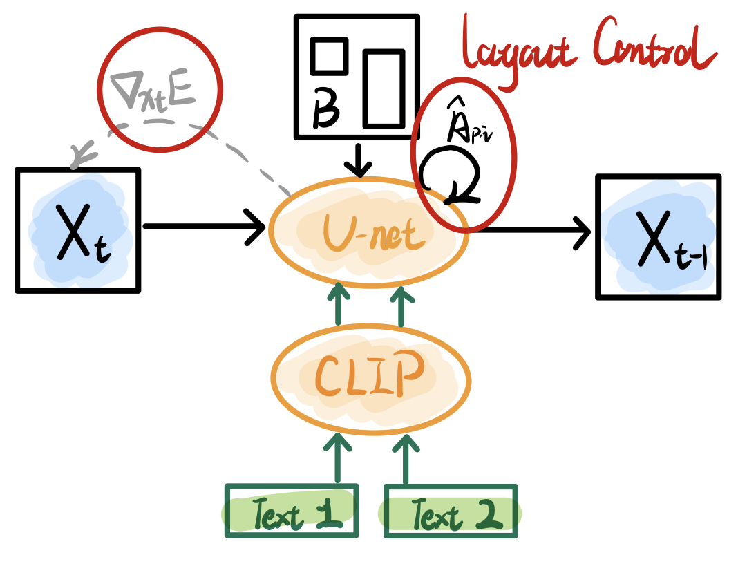
In particular, the forward guidance will modify the Cross-Attention of the specified text tokens (in each layer) to cluster them into the specified box:

$$ \hat{A_{p,i}}=(1-\lambda)A_{p,i}+\lambda g_p\sum_{j}A_{j,i} $$

Where $p$ is the position coordinate, $i$ is the index of the text token, $g_p$ is the gaussian weight in a specified box (sum of 1), and $\sum_{j}A_{j,i}$ is the sum of the entire CA Map. It means that the latter term in the equation will redistribute the attention weights according to the gaussian box.

Backward guidance defines a function to measure the CA concentration of a given token over a given box $B$:

$$ E(A,B,i)=\left(1-\frac{\sum_{p\in B}A_{p,i}}{\sum_{p}A_{p,i}}\right)^2 $$

We update the latent $x_t$ at the current time step with the gradient of this metric as shown in the figure.

According to the experimental results, the backward guidance is more effective (and of course consumes more running time). In addition, the author also integrates this method with Dreambooth and Text Inversion, which still achieve a good control effect.

Attend-and-Excite: Attention-Based Semantic Guidance for Text-to-Image Diffusion Models

-> Hila Chefer et al. ACM Trans. Graph. 2023

Similar to the observations in P2P, this paper assumes that if something is not generated as expected, the corresponding Cross-Attention should be increased. The difference, however, is that Attend-and-Excite establishes a certain metric as a loss function and backpropagates the gradient to excite the update of latents, rather than forcing up the corresponding value by direct re-weighting.

Specifically, we first need to select a few text tokens as the target to be enhanced (for example, the 2nd and 5th), calculate their corresponding average cross-attention ($A_t^2,A_t^5$), and then take the smallest peak of them as the loss:

$$ Loss=max\left(1-max(A_t^2),1-max(A_t^5)\right) $$

Finally, the latent is updated according to the gradient as $x_t^{\prime}=x_t-\alpha \nabla_{x_t} Loss$, which encourages the peak cross-attention of all selected text tokens to be as high as possible. Of course, there are several limitations of Attend-and-Excite as follows:

• Manually selecting the index of the enhanced token is not a convenient and perfect solution.
• If and only the excitation in the middle scale of Unet is effective. Because not all scales of cross-attention have semantic information and contribute semantically to the final generation.
• This involves too many hyperparameter settings, such as artificial thresholds that determine the number of backward updates during early iterations.

DragDiffusion: Harnessing Diffusion Models for Interactive Point-based Image Editing

-> Yujun Shi, et al. arXiv 2023

DragDiffusion is a direct extension of the famous DragGAN. Similarly, DragDiffusion can achieve image editing by dragging multiple points, and the principle behind it is the backward guidance for the generated path by gradient-based update.

As shown above, in addition to the regular diffusion denoising, the generated path in DragDiffusion contains two other mappings: Motion Supervision and Point Tracking. The loss function of Motion Supervision is shown as follows:

$$ \mathcal{L}\left(z_t^k\right)= \sum_{i=1}^n \sum_{q \in \Omega\left(h_i^k, r_1\right)}\lVert F_{q+d_i}\left(z_t^k\right)-\operatorname{sg}\left(F_q\left(z_t^k\right)\right) \rVert_1 +\lambda \lVert \left(z_{t-1}^k-\operatorname{sg}\left(z_{t-1}^0\right)\right) \odot(1-M) \rVert_1 $$

In simple terms, the former of this loss encourages feature movement at the patch level $F_{\Omega+d_i}(z_t^k) \gets F_{\Omega}(z_t^k)$, while the latter keeps the pixel values outside the mask nearly constant $(1-M)z_t^k \approx (1-M)z_t^{k+1}$.

Here $sg(\cdot)$ is the stop gradient operator, which makes the pixel values $F_{\Omega}(z_t^k)$ in the original patch are not affected by gradient descent directly. We can calculate the gradient and update the latent as follows:

$$ z_t^{k+1}=z_t^k-\eta \cdot \nabla_{z_t^k} \mathcal{L} $$

Point Tracking is used to rematch the location of the handle points, which is implemented directly using a nearest neighbor search:

$$ h_i^{k+1}=\underset{q \in \Omega\left(h_i^k, r_2\right)}{\arg \min }\left|F_q\left(z_t^{k+1}\right)-F_{h_i^k}\left(z_t\right)\right|_1 $$

Although this method directly follows DragGAN’s idea, the non-stationary iterative process of the Diffusion Models makes many hyperparameter different, and the author also abandons CFG to avoid large numerical errors.